ProtoFlow: Prototype-Guided Flow Matching for Multivariate Time Series Forecasting

📌 Highlights

ProtoFlow targets high-dimensional multivariate time series forecasting by combining vector-quantized representations with non-autoregressive rectified flow matching. Its key move is to initialize latent transport from learned prototype structure rather than a generic Gaussian prior.

The strongest empirical claim is broad main-result performance: the paper reports best or joint-best results in 18 out of 20 comparisons across five benchmarks and two horizons, while using only 3 ODE steps except 5 on Wikipedia.

The main caveat is that the efficiency story is not free: the paper reports 3.66-3.90x inference speedups over TSFlow, but also a 4.08-7.49x larger training-memory footprint.

Core claim: a VQ codebook can serve both as a latent discretizer and as a structured source prior for flow matching.
Main result: ProtoFlow reports strong CRPSsum and NRMSEsum performance on Electricity, Solar, Traffic, Taxi, and Wikipedia.
Key mechanism: prototype centers, empirical frequencies, and local variability initialize conditional transport in latent space.
Important limitation: reported reproducibility depends partly on future code availability and appendix-only details outside the main-body evidence.

🎯 Introduction

The paper addresses multivariate time series forecasting where many variables evolve over time, making high-dimensional joint predictive modeling difficult. The authors position generative models as a natural fit, but note that diffusion-based methods often require many denoising steps at inference.

The paper frames VAE and VQ latent forecasting as an efficiency-oriented alternative, but argues that existing VQ-based methods commonly use autoregressive token generation. Under teacher forcing, these models condition on ground-truth previous tokens during training but generated tokens at inference, creating rollout mismatch and error accumulation.

ProtoFlow’s objective is to replace autoregressive latent token rollout with non-autoregressive latent flow matching and to replace Gaussian flow initialization with a learned prototype prior derived from the VQ codebook. This makes the representation learner and the generative sampler more tightly coupled.

equation 2

Formula:

p(\mathbf{a}\mid\mathbf{c}) = \prod_{\ell=1}^{L} p(a_{\ell}\mid a_{<\ell},\mathbf{c}).

Meaning: Formalizes the autoregressive token-generation factorization that ProtoFlow aims to avoid.

🔬 Methodology

ProtoFlow first trains a VQ tokenizer over future target sequences. Given a target sequence, the encoder produces latent vectors, which are assigned to codebook entries by cosine similarity. The decoder reconstructs the target sequence from the quantized latent sequence, with a reconstruction-plus-commitment objective.

The second stage models future latent sequences with conditional rectified flow matching. Instead of drawing the source endpoint from a Gaussian, ProtoFlow constructs a mixture prior from codebook prototypes, empirical mixing weights, local basis directions, local scales, and a perturbation magnitude parameter. The source latent sequence is sampled independently across latent positions from this prototype prior.

The learned vector field is DiT-based and conditioned on historical context and future temporal features. At inference, ProtoFlow samples from the prototype prior, integrates the learned ODE over a small grid using Euler updates, and decodes the final latent into the forecast. The theoretical motivation is that a source prior closer to the target latent distribution in W2 distance should reduce the optimal rectified transport cost.

equation 6

Formula:

a_{\ell} = \underset{k\in\{1,\dots,K\}}{\arg\max} \frac{ \langle\hat{z}^{\ell},\mathcal{Z}_k\rangle }{ \|\hat{z}^{\ell}\|_2\|\mathcal{Z}_k\|_2 }, \qquad z_q^{\ell}=\mathcal{Z}_{a_{\ell}}. \label{eq:similarity_quantization}

Meaning: Defines similarity-based assignment into the VQ codebook.

equation 8

Formula:

\mathcal{L}_{\mathrm{VQ}} = \|\mathcal{X}_t-\hat{\mathcal{X}}_t\|_2^2 + \frac{\beta}{L} \sum_{\ell=1}^{L} \left( 1- \left\langle \hat{z}^{\ell}, \operatorname{sg}[z_q^{\ell}] \right\rangle \right), \label{eq:vq_loss_main}

Meaning: Trains the tokenizer to reconstruct targets while aligning encoder outputs with assigned codebook entries.

equation 9

Formula:

p_{\mathcal{Z}}(z) = \sum_{k=1}^{K} \pi_k\,p_k(z;\mu_k,B_k,\sigma_k,\gamma), \qquad \pi_k\geq 0,\quad \sum_{k=1}^{K}\pi_k=1, \label{eq:proto_prior}

Meaning: Defines the structured prototype prior used as the flow source distribution.

equation 4

Formula:

\mathcal{L}_{\mathrm{RFM}}(\theta) = \mathbb{E}_{\bm{c},t,\bm{x}_0,\bm{x}_1} \left[ \left\| \bm{v}_{\theta}(\bm{x}_t,t\mid\bm{c}) - (\bm{x}_1-\bm{x}_0) \right\|_2^2 \right]. \label{eq:rfm_objective}

Meaning: Optimizes the conditional velocity field for rectified flow matching.

📊 Experiments

The paper evaluates on five real-world high-dimensional MTS benchmarks: Solar, Electricity, Traffic, Taxi, and Wikipedia. Baselines include diffusion-based TimeGrad, CSDI, TSDiff, MG-TSD, DyDiff, and NsDiff, plus flow-based FlowTime and TSFlow. Metrics are CRPSsum for probabilistic forecasting and NRMSEsum for deterministic accuracy; lower values are better for both as reported by the error-reduction framing.

The main setup uses history length 96 and prediction lengths {48, 96}. Results are averaged over three runs, and forecasting metrics are computed from 100 generated samples per prediction window. The main table reports that ProtoFlow achieves best or joint-best performance in 18 out of 20 comparisons across the five datasets and two horizons.

The representation/generation ablation shows that VQ variants outperform VAE variants, and ProtoFlow improves over VQ + AR, ProtoFlow-G, and VAE + FM in the averaged 96-step results. The prototype-frequency ablation reports ProtoFlow at Avg. C-S 0.116 and Avg. NM-S 0.219, compared with ProtoFlow-G at 0.123 and 0.243 and ProtoFlow-uniform at 0.133 and 0.249.

Efficiency evidence is mixed but useful: Figure 2 reports faster convergence and 3.66-3.90x inference speedups over TSFlow, while also reporting 4.08-7.49x higher training memory. Figure 4 reports smaller W2 distance for ProtoFlow than ProtoFlow-G across ODE sampling budgets, supporting the prototype-prior transport argument.

tab:representation_results_summary

Caption: The comparison results of 96 prediction horizons with baselines regarding $ CRPS_ sum$ (C-S) and $ NRMSE_ sum$ (NM-S). AR: Auto-regressive Transformer and FM: Flow Matching .

Content:

2[2]* Method	2cElectricity	2cSolar	2cTraffic	2cTaxi	2cWikipedia	2cAvg.
	C-S	NM-S	C-S	NM-S	C-S	NM-S	C-S	NM-S	C-S	NM-S	C-S	NM-S
VAE + AR	0.421	0.544	1.154	2.618	1.005	1.511	0.337	0.448	0.130	0.169	0.609	1.058
VAE + FM	0.129	0.213	0.643	1.324	0.323	0.564	0.227	0.293	0.117	0.128	0.288	0.504
VQ + AR	0.037	0.054	0.347	0.833	0.066	0.084	0.205	0.322	0.108	0.121	0.153	0.283
ProtoFlow-G	0.019	0.037	0.305	0.717	0.036	0.058	0.159	0.287	0.096	0.114	0.123	0.243
ProtoFlow	0.015	0.022	0.284	0.638	0.034	0.054	0.157	0.281	0.092	0.101	0.116	0.219

Why It Matters: Shows the central 96-step representation and generation ablation.

tab:prototype_frequency

Caption: The forecasting performance with frequency-weighted prototype (ProtoFlow), uniform-weight prototype (ProtoFlow-uniform), and isotropic Gaussian priors (ProtoFlow-G) at a prediction length of 96.

Content:

2[2]* Method	2cElectricity	2cSolar	2cTraffic	2cTaxi	2cWikipedia	2cAvg.
	C-S	NM-S	C-S	NM-S	C-S	NM-S	C-S	NM-S	C-S	NM-S	C-S	NM-S
ProtoFlow-G	0.019	0.037	0.305	0.717	0.036	0.058	0.159	0.287	0.096	0.114	0.123	0.243
ProtoFlow-uniform	0.018	0.030	0.356	0.769	0.036	0.056	0.157	0.284	0.099	0.108	0.133	0.249
ProtoFlow	0.015	0.022	0.284	0.638	0.034	0.054	0.157	0.281	0.092	0.101	0.116	0.219

Why It Matters: Tests whether frequency-weighted prototypes outperform Gaussian and uniform prototype priors.

tab:results_codereset_main

Caption: Effects of codebook size on Stage 1 reconstruction MSE and $ NRMSE_ sum$ under frequency and uniform weighting at a 96-step prediction length.

Content:

2[2]*	3cElectricity	3cSolar	3cTraffic
	Frequency	Uniform	Stage1 MSE	Frequency	Uniform	Stage1 MSE	Frequency	Uniform	Stage1 MSE
Coodebook size
0.5em 64	0.039	0.044	red!157.76e-4	1.035	0.962	red!157.70e-4	0.113	0.105	red!155.82e-4
0.5em 128	0.030	0.032	7.13e-4	0.774	0.761	6.75e-4	0.062	0.066	5.23e-4
0.5em 256	0.022	0.030	yellow!156.02e-4	0.638	0.769	yellow!156.13e-4	0.054	0.056	yellow!154.78e-4
0.5em 512	0.031	0.033	yellow!156.01e-4	0.993	0.758	yellow!156.18e-4	0.056	0.057	yellow!154.69e-4

Why It Matters: Shows that insufficient codebook capacity hurts, while increasing from 256 to 512 can worsen forecasting despite little reconstruction gain.

fig:overall

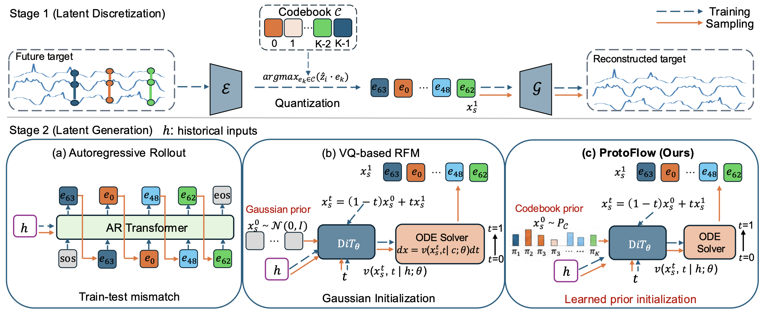
Caption: Illustration of our ProtoFlow. Stage 1 discretizes the future target sequence into compact latent tokens via similarity-based VQ latent modeling. Stage 2 compares three latent-generation paradigms under the same tokenized space: (a) Autoregressive rollout, which suffers from training--inference mismatch; (b) Gaussian-initialized flow matching, which starts transport from an unstructured prior; and (c) The proposed ProtoFlow, which initializes conditional rectified flow from a learned codebook prior for latent flow matching generation. The future time features $ y^c$ is omitted here.

Why It Matters: It visually anchors the two-stage design and contrasts ProtoFlow with autoregressive rollout and Gaussian-initialized flow matching.

fig:efficiency

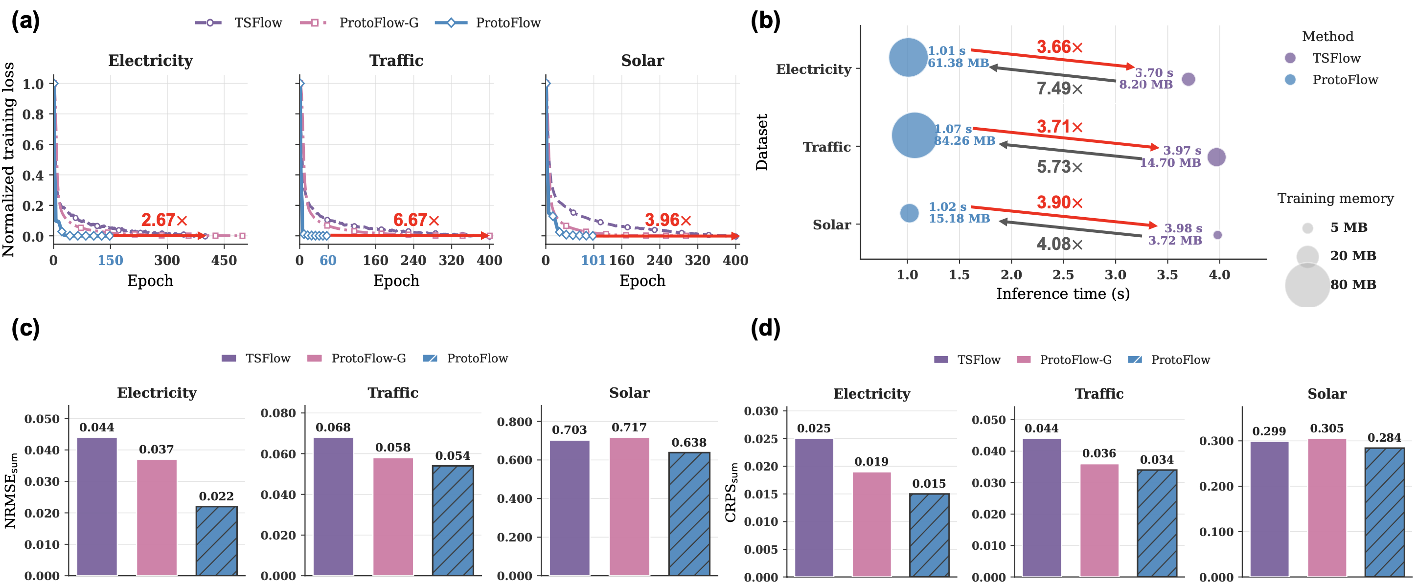
Caption: Comparison of training convergence (a), inference efficiency, training memory (b), and forecasting performance (c-d) on Electricity, Traffic, and Solar with a prediction length of 96.

Why It Matters: It links the prototype prior to training stabilization, inference speed, memory cost, and forecasting accuracy on three core benchmarks.

fig:codebook_size

Caption: Effects of codebook size on ProtoFlow at the 96-step prediction length.

Why It Matters: It shows that codebook capacity must be tuned jointly with prior estimation; larger codebooks are not automatically better.

fig:sampling

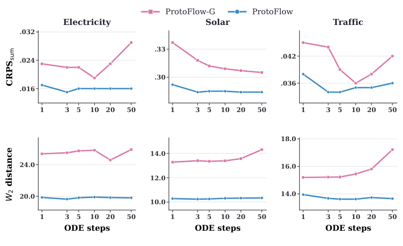
Caption: Effect of ODE sampling steps on 96-step probabilistic forecasting performance and $W_2$ transport distance for ProtoFlow and ProtoFlow-G.

Why It Matters: It supports the claim that prototype initialization reduces transport distance and maintains strong few-step forecasting performance.

🔮 Conclusion

The paper concludes that prototype-prior flow matching can make generative MTS forecasting more efficient by reusing learned codebook structure as the source distribution for latent transport. The reported evidence supports strong accuracy with few ODE steps, earlier flow-matching stabilization, and reduced sampling-budget sensitivity relative to Gaussian initialization.

For builders, the practical takeaway is not just to tokenize time series, but to preserve and exploit codebook statistics after tokenizer training. In ProtoFlow, representation learning and source-prior design are coupled rather than treated as independent modules.

🛠️ Future Research Improvements

A natural next research direction is stronger reproducibility: the main body states that code will be publicly available upon acceptance, but builders need released training code, data preprocessing, and hyperparameter details to verify the reported speed-memory-accuracy tradeoff.

The memory footprint deserves further optimization. The paper reports faster inference than TSFlow but also 4.08-7.49x higher training memory, so future work could explore lighter tokenizer or DiT configurations, prior distillation, or memory-efficient training schedules.

The codebook-prior design could be extended beyond fixed empirical frequencies. The ablations show interactions among codebook size, frequency weighting, and forecasting quality, suggesting room for adaptive priors that account for dataset size, seasonal regimes, or conditioning context.

🏭 Potential Industry Use Scenarios

ProtoFlow is most credible for high-dimensional forecasting settings where inference latency matters and probabilistic forecasts are useful: energy demand, traffic volume, taxi demand, and web-traffic forecasting are directly represented by the paper’s benchmark set.

An operations team could use the method when it needs many sample forecasts per prediction window but cannot afford diffusion-style denoising budgets. The reported use of 3 to 5 ODE steps is attractive for repeated forecasting workloads, provided the training-memory cost is acceptable.

The method may be especially useful when a learned latent codebook already captures recurring system states, such as demand regimes, traffic patterns, or aggregate web activity modes. The uncertainty is deployment robustness: the main-body evidence does not verify distribution shift, online updating, or production monitoring behavior.

💬 Critical Analysis

ProtoFlow’s strength is a clean alignment between the problem diagnosis and the method: AR token forecasting has rollout mismatch, Gaussian flow priors are unstructured, and VQ codebooks already contain learned latent prototypes. Using those prototypes as the flow source prior is technically coherent and well supported by the ablations in the main body.

The experimental package is broad enough to be meaningful: five benchmarks, diffusion and flow baselines, two horizons, representation/generation ablations, codebook-size analysis, prototype-frequency analysis, and sampling-step sensitivity. The strongest builder-facing table is the 96-step ablation, where ProtoFlow improves the average C-S and NM-S values over VQ + AR, ProtoFlow-G, and ProtoFlow-uniform.

The main weakness is the tradeoff profile and verification gap. The paper reports faster inference but substantially higher training memory than TSFlow, and public code is not available in the main-body evidence beyond the statement that it will be released upon acceptance. Also, some important reproducibility details are deferred to appendices, which are outside the stated evidence boundary here.

Overall, the paper is a strong candidate for builders exploring efficient probabilistic forecasting, but it should be treated as a method to reproduce carefully rather than a drop-in claim. The central question to verify is whether the prototype prior still helps under each builder’s own data scale, regime shifts, and memory constraints.

Original Abstract

Generative modeling has shown strong promise for multivariate time mseries (MTS) forecasting, especially scale to high-dimensional settings. Diffusion-based methods achieve competitive performance but typically require many sampling steps at inference. VAE-based non-iterative forecasting frameworks have therefore emerged as an efficient alternative. Within this line of work, vector quantization (VQ) enables controllable latent space modeling by mapping multivariate series into compact discrete representations. Existing VQ-based forecasting methods, however, typically rely on autoregressive (AR) token generation, which suffers from exposure bias and training-inference mismatch. Flow matching provides an efficient non-autoregressive alternative for latent forecasting, but existing formulations usually initialize transport from a generic Gaussian prior. We instead observe that the trained VQ codebook already captures representative latent prototypes and can thus serve as a more informative prior for flow matching. Based on this insight, we propose ProtoFlow, a forecasting framework that combines vector-quantized autoencoding with Prototype-prior Flow matching. Our method first maps multivariate sequences into a discrete latent space, then constructs a structured prior from the learned codebook, and finally learns a DiT-based rectified flow to transport samples from this prior to future latent representations conditioned on historical observations. By replacing generic noise initialization with a learned prototype prior, ProtoFlow avoids the rollout mismatch of AR token prediction and promotes faster training convergence. Extensive experiments on benchmark datasets show that it consistently achieves superior forecasting performance with efficient inference.